
In this post, I will show how directly derive the Gaussian process formulation of nonlinear regression from probabilistic linear regression model. Doing this, some common misunderstanding of GP will be clear.
First, for reference purpose, let’s write down the probabilistic formulation for linear regression.
0.1. Probabilistic Linear Regression
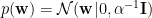
For a linear model

where the noise 


Assuming the priors is
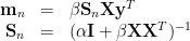
The posterior then is

where
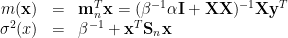
Given new samle 

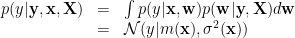
where
These are textbook illustration which can be found in PRML.
To deal with the bias term 

one way is to use the augment variable trick ![{\tilde{\mathbf{x}}=[1,\mathbf{x}^T]^T}](https://s0.wp.com/latex.php?latex=%7B%5Ctilde%7B%5Cmathbf%7Bx%7D%7D%3D%5B1%2C%5Cmathbf%7Bx%7D%5ET%5D%5ET%7D&bg=ffffff&fg=000000&s=0&c=20201002)


0.2. Gaussian Process
Textbooks often directly present you the Gaussian process, then show the predictive distribution of GP is actually equivalent to linear regression when linear kernel used. However, since there is equivalence, we should be able to derive from one to another. Usually your textbook does not tell you how.
Here is the PRML way to present the GP (where we switch the symbols for consistency sake)
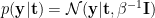
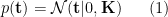
Then marginalizing out 
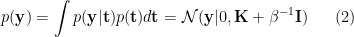
![\displaystyle p(y|\mathbf{y})=\frac{p([y,\mathbf{y}])}{p(\mathbf{y})}=\mathcal{N}(y|m(\mathbf{x}),\sigma^2(\mathbf{x})) \ \ \ \ \ (3)](https://s0.wp.com/latex.php?latex=%5Cdisplaystyle++p%28y%7C%5Cmathbf%7By%7D%29%3D%5Cfrac%7Bp%28%5By%2C%5Cmathbf%7By%7D%5D%29%7D%7Bp%28%5Cmathbf%7By%7D%29%7D%3D%5Cmathcal%7BN%7D%28y%7Cm%28%5Cmathbf%7Bx%7D%29%2C%5Csigma%5E2%28%5Cmathbf%7Bx%7D%29%29+%5C+%5C+%5C+%5C+%5C+%283%29&bg=ffffff&fg=000000&s=0&c=20201002)
where
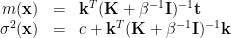
where 


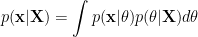
Actually, there is another way that we can first marginalize parameter 
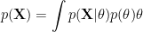
By integrate out the parameter
![\displaystyle p(\mathbf{x}|\mathbf{X})=\frac{p([\mathbf{x},\mathbf{X}])}{p(\mathbf{X})}](https://s0.wp.com/latex.php?latex=%5Cdisplaystyle+p%28%5Cmathbf%7Bx%7D%7C%5Cmathbf%7BX%7D%29%3D%5Cfrac%7Bp%28%5B%5Cmathbf%7Bx%7D%2C%5Cmathbf%7BX%7D%5D%29%7D%7Bp%28%5Cmathbf%7BX%7D%29%7D&bg=ffffff&fg=000000&s=0&c=20201002)
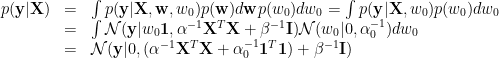
To derive GP formulation of regression from linear regression, one way is to first marginalize out 

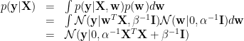
This marginal likelihood is equivalent to (2). Therefore you can see, in order to establish the exact equivalence, the kernel matrix should be 
![\displaystyle p(y|\mathbf{y},[\mathbf{x},\mathbf{X}])=\frac{p([y,\mathbf{y}]|[\mathbf{x},\mathbf{X}])}{p(\mathbf{y}|\mathbf{X})}=\mathcal{N}(y|m(\mathbf{x}),\sigma^2(\mathbf{x}))](https://s0.wp.com/latex.php?latex=%5Cdisplaystyle+p%28y%7C%5Cmathbf%7By%7D%2C%5B%5Cmathbf%7Bx%7D%2C%5Cmathbf%7BX%7D%5D%29%3D%5Cfrac%7Bp%28%5By%2C%5Cmathbf%7By%7D%5D%7C%5B%5Cmathbf%7Bx%7D%2C%5Cmathbf%7BX%7D%5D%29%7D%7Bp%28%5Cmathbf%7By%7D%7C%5Cmathbf%7BX%7D%29%7D%3D%5Cmathcal%7BN%7D%28y%7Cm%28%5Cmathbf%7Bx%7D%29%2C%5Csigma%5E2%28%5Cmathbf%7Bx%7D%29%29&bg=ffffff&fg=000000&s=0&c=20201002)
where

Then you can substitute the inner product in above formulation with kernel to get nonlinear regression.
Be careful when you see a Gaussian process 


Dealing with bias in GP is very tricky. One way is to use the augment kernel 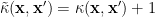

Another way is to use the centering kernel
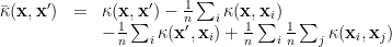
then define a Gaussian process 
One might think that we can derive the GP from a probabilistic linear regression formulation which is translation invariant. However, it is not easy. To see why, we explicitly marginalize the
As indicated in previous section, the data centering is equivalent to make 
To contruct a GP for regression which is translation invariant is superisingly non-trivial. How to solve the dilemma is still bothering me. I cannot figure out a way to have a GP, when used for regression, the solution of which is translation invariant. I hope there is a easier way to do it. Maybe the reality is that you can not! Any suggestion is welcome.

Pingback: Undocumented Machine Learning | Machine Learning Rumination